
SolarMamba: Adaptive Hierarchical Fusion of Vision State-Space Models and Temporal Networks (Ongoing)
Overview
Most multi-modal forecasting architectures treat all input modalities equally regardless of scene conditions, concatenating or adding features without asking whether the visual signal is actually informative at any given moment. Under overcast skies or heavy fog, an all-sky camera captures near-uniform texture; the image carries little useful information, and the model should rely on temporal momentum instead. Under partially cloudy skies, cloud edge positions are highly predictive, and the visual pathway should dominate.
SolarMamba addresses this directly. The core contribution is LadderFusion, a lightweight mechanism that injects an external temporal embedding as a channel-wise gate into each stage of a visual backbone, dynamically modulating how much the model trusts its own visual features based on current atmospheric state. This is paired with a MambaVision-B visual backbone and a Pyramid Temporal CNN, forming a unified architecture.
The Core Problem: When Should a Model Trust Its Eyes?
Standard fusion approaches — concatenation, additive fusion, SE-Net self-gating share a fundamental limitation: the gate is a function only of the visual features themselves. A gate that cannot observe signals outside the visual pathway cannot respond to atmospheric state that is not visually manifest. A uniformly grey overcast sky looks identical whether it has been overcast for 5 minutes or 5 hours, yet these two states have very different persistence profiles.
LadderFusion solves this by conditioning the gate exclusively on the external temporal signal a 40-minute meteorological history that encodes atmospheric momentum independently of what the camera sees.
Architecture
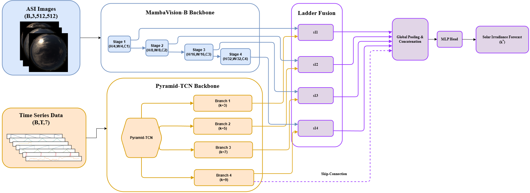
SolarMamba integrates three synchronised processing streams:
All-Sky Image (512×512×3)          Meteorological Time-Series (40×7)
        │                                        │
        ▼                                        ▼
  MambaVision-B                           PyramidTCN
  ┌──────────────┐                    ┌──────────────────┐
  │ Stage 1: CNN │◄── LadderFusion ───│ Branch 1: k=3    │
  │ Stage 2: CNN │◄── LadderFusion ───│ Branch 2: k=5    │
  │ Stage 3: SSM │◄── LadderFusion ───│ Branch 3: k=7    │
  │ Stage 4: SSM │◄── LadderFusion ───│ Branch 4: k=9    │
  └──────────────┘                    └──────────────────┘
        │                                        │
        ▼                                        ▼
   Cross-Level Spatiotemporal Fusion (4×4 mixing matrix)
        │
        ▼
   Global Average Pool → Concat with Temporal Skip (2944-dim)
        │
        ▼
   MLP Head → k* predictions for 6 horizons (10–60 min)
MambaVision-B Visual Backbone
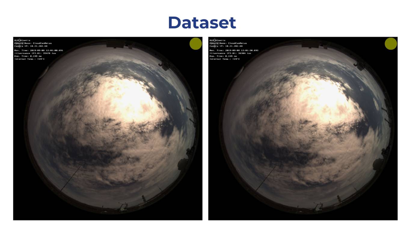
The visual stream processes 512×512 all-sky images through a four-stage hierarchical pipeline. Stages 1 and 2 use standard residual convolutions to extract low-level spatial features — cloud edges, textures, and local intensity patterns — at high spatial resolution. Stages 3 and 4 transition to MambaVision Mixer blocks, which interleave selective State Space Model (SSM) layers with multi-head self-attention.
| Stage | Operator | Resolution | Channels | Complexity |
|---|---|---|---|---|
| 1 | Residual Conv | H/4 × W/4 | 256 | O(HW) |
| 2 | Residual Conv | H/8 × W/8 | 512 | O(HW) |
| 3 | MambaVision + Attn | H/16 × W/16 | 1024 | O(n) |
| 4 | MambaVision + Attn | H/32 × W/32 | 1024 | O(n) |
The SSM’s O(n) recurrent computation is a critical design choice. At 512×512 input resolution, standard self-attention would require O(1,024²) ≈ 1M operations per layer in Stages 3–4; Mamba reduces this to O(1,024). This makes the full 512×512 pipeline feasible for real-time deployment. The backbone is initialised from ImageNet-1K pretrained weights.
Pyramid Temporal CNN (PyramidTCN)
The temporal stream processes a 40-step (40-minute) lookback window of 7 meteorological features: clear-sky index k*, temperature, pressure, solar zenith angle, solar azimuth angle, sin(hour), and cos(hour). Features are first projected to a 128-dimensional embedding, then processed in parallel by four 1D convolutional branches with kernel sizes k = [3, 5, 7, 9]:
- Branch 1 (k=3): 3-minute receptive field — high-frequency fluctuations and immediate momentum
- Branch 2 (k=5): 5-minute receptive field — cloud edge transit dynamics
- Branch 3 (k=7): 7-minute receptive field — partial cloud transition patterns
- Branch 4 (k=9): 9-minute receptive field — low-frequency diurnal trends and weather system evolution
Each branch outputs a fixed 128-dimensional vector via adaptive average pooling, matched to the corresponding MambaVision-B stage for LadderFusion gating.
LadderFusion
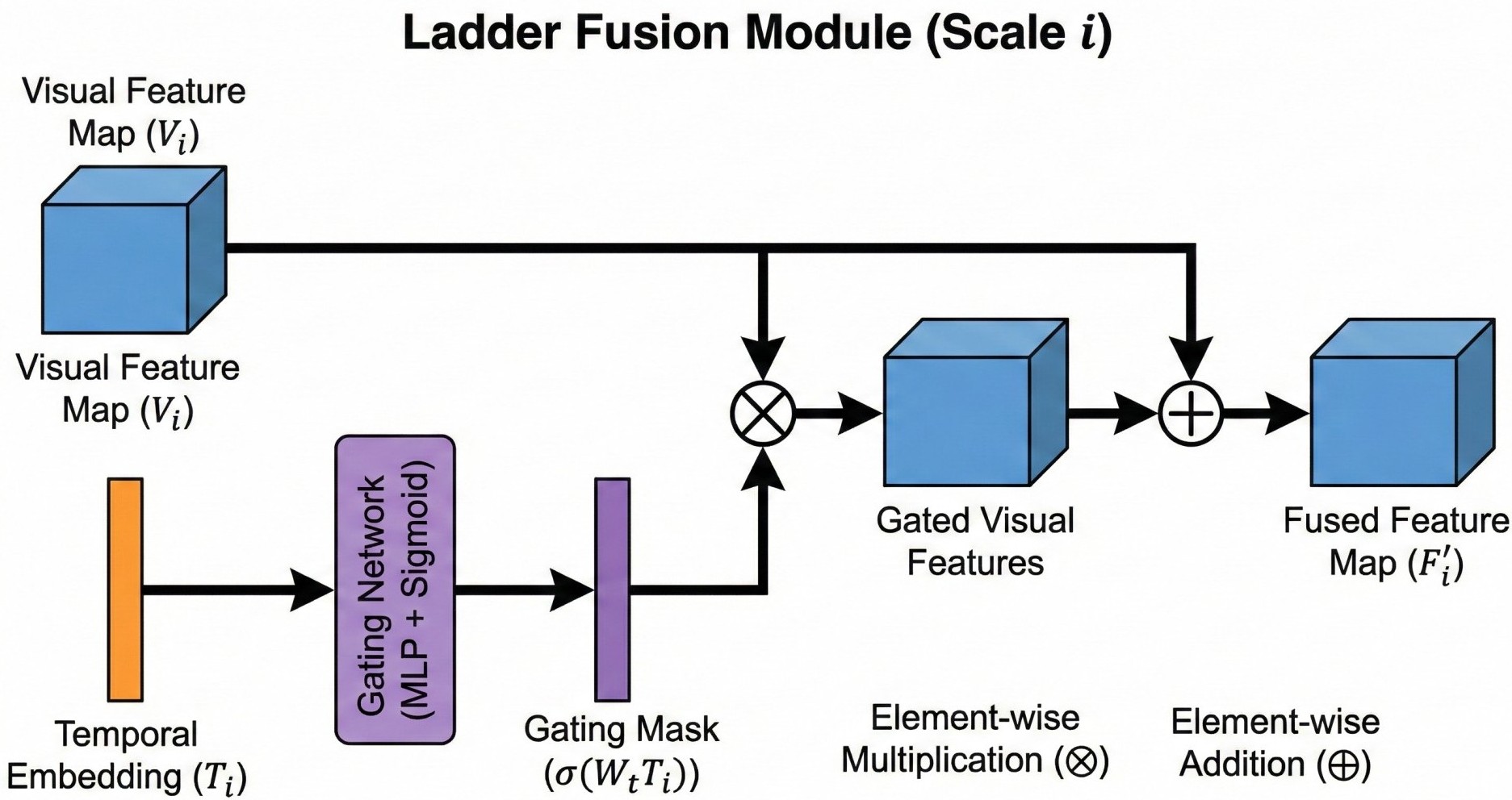
For each backbone stage i, LadderFusion takes the temporal embedding tⱼ ∈ ℝ¹²⁸ from the matched PyramidTCN branch and computes a channel-wise gate over the visual feature map fᵢ ∈ ℝ^(Cᵢ × Hᵢ × Wᵢ):
F_gate  = W · t_j                  (linear projection: 128 → Cᵢ)
α_i     = σ(F_gate)  ∈ [0, 1]^Cᵢ  (sigmoid → gate values)
F_fused = f_i ⊙ α_i + f_i          (modulate + residual bypass)
The residual term + f_i is non-optional. Without it, gates collapsing to zero would discard all visual structure — including low-level cloud edge features that remain informative even under partial overcast. The bypass ensures the model degrades gracefully rather than catastrophically when visual information is absent.
What makes LadderFusion different from SE-Net: SE-Net gates are conditioned on the visual features themselves — they re-weight channels based on what the image shows. LadderFusion gates are conditioned on an entirely external signal. A gate that cannot see outside the visual pathway cannot respond to atmospheric state that is not visible. This distinction is the operative mechanism behind LadderFusion’s performance gains.
LadderFusion is applied at all four backbone stages simultaneously, injecting temporal context at every level of the visual hierarchy — from low-level edge features at Stage 1 to high-level semantic cloud representations at Stage 4.
Cross-Level Spatiotemporal Fusion
Standard fusion assumes strict level-to-level correspondence: Stage 1 temporal features gate Stage 1 visual features, and so on. This is physically limiting. Short-duration shadow transients encoded in shallow visual features may be more reliably interpreted in conjunction with deeper temporal context capturing slow-moving weather system state.
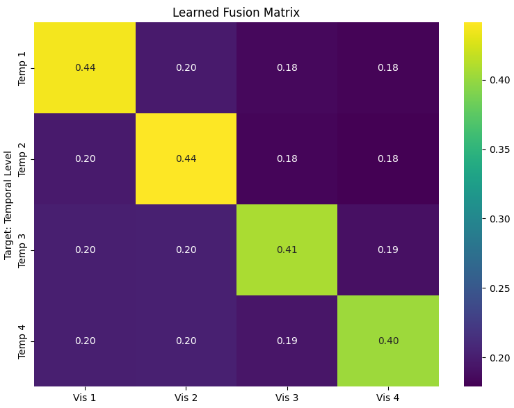
To address this, a Learnable 4×4 Mixing Matrix M allows cross-scale associations to be discovered data-driven. M is initialised as the identity matrix (equivalent to standard level-aligned fusion at training start) and learns off-diagonal weights only when cross-level interactions reduce prediction error. After convergence, the matrix reveals that Stage-1 visual features receive meaningful contributions from Stage-3 and Stage-4 temporal embeddings — confirming that slow atmospheric dynamics influence how low-level cloud boundary features should be weighted.
Prediction Head
After four stages of LadderFusion, each gated feature map is global-average-pooled to a channel vector. The four vectors are concatenated with a direct temporal skip connection from PyramidTCN Branch 1:
z = [p₁(256); p₂(512); p₃(1024); p₄(1024); t₁(128)] = 2944-dim vector
This skip connection is architecturally essential: if all LadderFusion gates suppress visual features under extreme overcast, the temporal skip ensures the head still has direct access to the meteorological trajectory for persistence-based forecasting.
The head is a two-layer MLP:
LayerNorm → Dropout(0.5) → Linear(2944→256) → GELU → Dropout(0.5) → Linear(256→6)
outputting simultaneous k* predictions for all six horizons: {10, 20, 30, 40, 50, 60} minutes.
Physics-Informed Preprocessing
Rather than predicting raw GHI directly, SolarMamba targets the clear-sky index:
k*(t) = GHI(t) / (GHI_cs(t) + ε) ∈ [0, 1.2]
where GHI_cs is the theoretical clear-sky irradiance from the Ineichen model (AOD = 1.0), computed via pvlib. This normalisation removes the site-specific diurnal baseline, making k* statistically homogeneous across all four datasets regardless of latitude or season — the key property that enables cross-site generalisation without fine-tuning.
Solar zenith angle (SZA) and azimuth angle are explicitly provided as temporal features, grounding the model in deterministic geometric context. Night samples (SZA > 85°) are excluded, reducing the dataset from 1.525M to 660K daylight samples and removing trivially zero-irradiance records.
Datasets
Evaluated across four publicly available benchmarks spanning three Köppen climate classifications — no site-specific fine-tuning applied:
| Dataset | Location | Climate | Period | Target |
|---|---|---|---|---|
| NREL | Golden, Colorado | BSk — Semi-Arid | 2017–2022 | GHI (10-min images) |
| Folsom | Folsom, California | Csa — Mediterranean | 2014–2016 | GHI (1-min images) |
| SIRTA | Palaiseau, France | Cfb — Temperate Oceanic | 2017–2019 | GHI (1-min images) |
| Stanford | Stanford, California | Csb — Coastal Temperate | 2017–2019 | PV power (1-min images) |
All datasets use a chronological 70/15/15 train/validation/test split.
Implementation
# Core configuration
input_resolution: 512 × 512 × 3
temporal_lookback: T = 40 steps (1-min resolution)
temporal_features: C = 7
forecast_horizons: [10, 20, 30, 40, 50, 60] min
backbone: MambaVision-B (ImageNet-1K pretrained)
fusion: LadderFusion × 4 stages (Xavier uniform init)
optimiser: AdamW (lr=3×10⁻⁴, weight_decay=0.01)
schedule: Cosine decay + 10-epoch linear warmup
training: 100 epochs, early stopping (patience=15 on val RMSE)
dropout: 0.5 (head layers)
hardware: NVIDIA A100 40GB / V100 32GB
Visual Results
Acknowledgments
This work is conducted under the guidance of Prof. Roshan Godaliyadda and Prof. Parakrama Ekanayake, MARC, University of Peradeniya and the Department of Electrical and Electronic Engineering, University of Peradeniya.